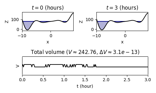
One dimension shallow water, steady lake validation case.

A steady lake is modelised by shallow water equation.

The model reads as

\[\begin{split}\begin{cases} \frac{\partial h}{\partial t} + \frac{\partial h}{\partial x} &= 0 \\ \frac{\partial u}{\partial t} + u\,\frac{\partial u}{\partial x} &= -g\,\frac{\partial h}{\partial x} \end{cases}\end{split}\]

The initial condition is a uniform fluid altitude on a curvy bottom. We expect the fluid altitude to remain constant as well as the total volume of fluid.

The finite difference being unable ensure quantity conservation, this very simple case can fail as the numerical error stacks, leading to wave that appears and propagate.

import pylab as pl
import numpy as np
from skfdiff import Model
from scipy.integrate import trapz

shallow = Model(
    ["-dxq", "-(g*h*dxh + 2*q*dxq/h - q**2*dxh/h**2 + g * h * dxZ - k * dxxh) * eps"],
    ["h(x)", "q(x)"],
    ["g", "k", "eps(x)", "Z(x)"],
    boundary_conditions="periodic",
)

x, dx = np.linspace(-10, 8, 500, retstep=True)
Z = x ** 2 * np.sin(x) + 3 * x + 80

h = 80 - Z

ini_fields = shallow.Fields(x=x, h=h, q=x * 0, Z=Z, g=9.81, k=0, eps=np.ones(x.size))

This hook ensure proper computation in dry places.

def dry_hook(t, fields):
    fields["eps"] = "x", np.where(fields.h <= 1, 0, 1)
    fields["q"] = "x", np.where(fields.h <= 0, 0, fields.q)
    return fields


simul = shallow.init_simulation(
    fields=ini_fields,
    hook=dry_hook,
    t=0,
    dt=60,
    tmax=3600 * 3,
    id="steady_lake",
    tol=1e-1,
)

container = simul.attach_container()
simul.run()

data = container.data.copy()
data["h"] = data["h"].where(data.h > 0)
data["q"] = data["q"].where(data.h > 0)
data["eta"] = data.h + data.Z
data["V"] = "t", trapz(data.h.where(data.h >= 0, other=0), x=data.x)

fig = pl.figure(figsize=(5, 3))

ax = pl.subplot2grid((2, 2), (0, 0))
pl.sca(ax)
data["eta"].isel(t=0).plot(color="navy")
pl.fill_between(
    data.x, data["eta"].isel(t=0), data["Z"].isel(t=0), color="navy", alpha=0.3
)
data["Z"].isel(t=0).plot(color="black")
pl.xlim(data["x"].min(), data["x"].max())
pl.title("$t=0$ (hours)")

ax = pl.subplot2grid((2, 2), (0, 1))
pl.sca(ax)
data["eta"].isel(t=-1).plot(color="navy")
data["Z"].isel(t=-1).plot(color="black")
pl.fill_between(
    data.x, data["eta"].isel(t=-1), data["Z"].isel(t=-1), color="navy", alpha=0.3
)
pl.xlim(data["x"].min(), data["x"].max())
pl.title("$t=3$ (hours)")

ax = pl.subplot2grid((2, 2), (1, 0), colspan=2)
pl.sca(ax)
pl.plot(data["t"] / 3600, data["V"], color="black")
pl.ylim(242.7621835042269, 242.7621835042272)
pl.xlim((data["t"] / 3600).min(), (data["t"] / 3600).max())
pl.title(r"Total volume ($V \approx 242.76$, $\Delta V \approx 3.1e-13$)")
pl.xlabel("t (hour)")
pl.ylabel("V")

pl.tight_layout()
pl.show()