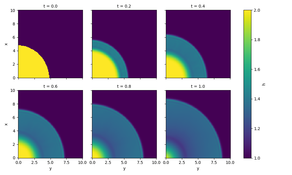
Two dimension dam break study case.

The dam break is known to be difficult to solve numericaly due to its initial discontinuity.

It simulate the behavior of a column of fluid confined by wall. At the initial time, the wall is removed, leading to a wave propagation.

The shallow water equation will modelise the fluid dynamic and is described by the equation below :

\[\begin{split}\begin{cases} \frac{\partial h}{\partial t} + \frac{\partial h}{\partial x} + \frac{\partial h}{\partial y} &= 0 \\ \frac{\partial u}{\partial t} + u\,\frac{\partial u}{\partial x} + v\,\frac{\partial u}{\partial y} &= -g\,\frac{\partial h}{\partial x}\\ \frac{\partial v}{\partial t} + u\,\frac{\partial v}{\partial x} + v\,\frac{\partial v}{\partial y} &= -g\,\frac{\partial h}{\partial y} \end{cases}\end{split}\]

This example will focus on 2D dam break, with wall at the boundaries (simulated as no-flux boundary) and a curved dam.

import skfdiff as sf
import numpy as np
from scipy.ndimage import gaussian_filter
import pylab as plt

Model definition

The PDE has to be written. It is just the RHS of the model as defined earlier written as \(\frac{\partial U}{\partial t} = F(U)\). Moreover, in that specific case, we will also specify that the advective terms has to be discretized with an upwind scheme to mitigate the numerical errors that will occur at the discontinuity. This is especially needed as we do not have diffusion at all in the model that could smooth the numerical errors.

Boundary conditions

The boundary condition will be empty, and will fallback to scikit-fdiff default (no-flux condition at every boundaries).

shallow_2D = sf.Model(
    [
        "-dx(h * u) - dy(h * v)",
        "-upwind(u, u, x, 2) - upwind(v, u, y, 2) - g * dxh",
        "-upwind(u, v, x, 2) - upwind(v, v, y, 2) - g * dyh",
    ],
    ["h(x, y)", "u(x, y)", "v(x, y)"],
    parameters=["g"],
)

Filter post-process

As the discontinuity will be still harsh to handle by a “simple” finite difference solver (a finite volume solver is usually the tool you will need), we will use a gaussian filter that will be applied to the fluid height. This will smooth the oscillation (generated by numerical errors). This can be seen as a way to introduce numerical diffusion to the system, often done by adding a diffusion term in the model. The filter has to be carefully tuned (the same way an artificial diffusion has its coefficient diffusion carefully chosen) to smooth the numerical oscillation without affecting the physical behavior of the simulation.

def filter_instabilities(simul):
    simul.fields["h"] = ("x", "y"), gaussian_filter(simul.fields["h"], 0.46)

Initial condition

A quarter of a circle has been chosen as initial condition, with the fluid inside the bottom left of the domain being higher that the rest of the domain.

x = y = np.linspace(0, 10, 128)
xx, yy = np.meshgrid(x, y, indexing="ij")
u = v = np.zeros_like(xx)
h = np.where(xx ** 2 + yy ** 2 < 5 ** 2, 2, 1)
fields = shallow_2D.Fields(x=x, y=y, u=u, v=v, h=h, g=9.81)

Simulation configuration

The only subtility is that the time-stepping will be desactivated. The problem does not need to have a variable time-step, and a properly chosen one will garanty us a good resolution.

simul = shallow_2D.init_simulation(fields, 0.01, tmax=1, time_stepping=False)
simul.add_post_process("filter", filter_instabilities)
container_shallow = simul.attach_container()
t_max, fields_final = simul.run()

container_shallow.data.h[::20].plot(col="t", col_wrap=3)
plt.savefig("../docs/_static/2D_dam_break.png")