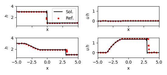
One dimension shallow water, dam break case.

This validation example use the shallow water equation to model a dam sudden break. The two part of the domain have different fluid depth and are separated by a well. A a certain instant, the wall disappear, leading to a discontinuity wave in direction of the lower depth, and a rarefaction wave in direction of the higher depth.

The model reads as

\[\begin{split}\begin{cases} \frac{\partial h}{\partial t} + \frac{\partial h}{\partial x} &= 0 \\ \frac{\partial u}{\partial t} + u\,\frac{\partial u}{\partial x} &= -g\,\frac{\partial h}{\partial x} \end{cases}\end{split}\]

and the results are validated on the Randall J. LeVeque book (LeVeque, R. (2002). Finite Volume Methods for Hyperbolic Problems (Cambridge Texts in Applied Mathematics). Cambridge: Cambridge University Press. doi:10.1017/CBO9780511791253).

import pylab as pl
import pandas as pd
from skfdiff import Model, Simulation
import numpy as np
from scipy.signal import savgol_filter

shallow_water = Model(["-dx(h * u)", "-upwind(u, u, x, 1) - dxh"], ["h(x)", "u(x)"])

Filter post-process

As the discontinuity will be still harsh to handle by a “simple” finite difference solver (a finite volume solver is usually the tool you will need), we will use a gaussian filter that will be applied to the fluid height. This will smooth the oscillation (generated by numerical errors). This can be seen as a way to introduce numerical diffusion to the system, often done by adding a diffusion term in the model. The filter has to be carefully tuned (the same way an artificial diffusion has its coefficient diffusion carefully chosen) to smooth the numerical oscillation without affecting the physical behavior of the simulation.

def filter_instabilities(simul):
    simul.fields["h"] = ("x",), savgol_filter(simul.fields["h"], 21, 4)


x, dx = np.linspace(-5, 5, 1000, retstep=True)
h = np.where(x < 0, 3, 1)
u = x * 0

init_fields = shallow_water.Fields(x=x, h=h, u=u)

simul = Simulation(
    shallow_water,
    t=0,
    dt=0.02,
    tmax=2,
    fields=init_fields,
    time_stepping=False,
    id="dambreak",
)

simul.add_post_process("filter", filter_instabilities)

container = simul.attach_container()

simul.run()

data = container.data.sel(t=[0, 0.5, 2], method="nearest")
fig, axs = pl.subplots(2, 2, sharex="all", figsize=(5.5, 2.5))
for i, t in enumerate(data.t):
    if i == 1:
        continue
    if i == 2:
        pl.sca(axs[i - 1, 0])
    else:
        pl.sca(axs[i, 0])
    data.sel(t=t).h.plot(color="black", label="Sol.")
    ref_data = pd.read_csv("valid_randall/dam_h%i.csv" % i)
    pl.scatter(ref_data.x, ref_data.h, color="red", marker=".", label="Ref.")
    pl.title("")
    pl.ylabel(r"$h$")
    pl.xlim(-5, 5)
    pl.ylim(0.5, 4)
    if i == 0:
        pl.legend()
    if i == 2:
        pl.sca(axs[i - 1, 1])
    else:
        pl.sca(axs[i, 1])
    (data.sel(t=t).h * data.sel(t=t).u).plot(color="black", label="Sol.")
    ref_data = pd.read_csv("valid_randall/dam_hu%i.csv" % i)
    pl.scatter(ref_data.x, ref_data.h, color="red", marker=".", label="Ref.")
    pl.title("")
    pl.ylabel(r"$u\,h$")
    pl.xlim(-5, 5)
    pl.ylim(-0.5, 1.5)
    pl.tight_layout()

pl.show()