Overview

Write your model

scikit-fdiff use Sympy to process the mathematical model given by the user.

It should be able to solve every systems that can be written as

\[\frac{\partial U}{\partial t} = F(U, \partial_{x,y,z...} U)\]

U being a single dependent variable or a list of dependent variables. The time t is a mandatory independent variable (and is hard-coded), but you can have any other spatial independent variables (x, y, z, r…), as long as they are written with only one character.

We can use the 2D heat diffusion as example:

\[\frac{\partial T(x,y)}{\partial t} = k\,(\partial_{xx} T + \partial_{yy} T)\]

You only have to write the right-hand side (rhs) : the python code will look like

>>> from skfdiff import Model
>>> model = Model("k * (dxxT + dyyT)",
...               "T(x, y)", parameters="k")

Be careful, the (x, y) after the dependent variable is mandatory. If not set, scikit-fdiff will consider a one-dimension problem (T(x)).

You can also set a variable parameter that can depend on coordinate by specifying its coordinate dependency (as k(x, y)). You will then be able to use its derivative in the equation (aka, use dxk, dyk… in the evolution equations).

from skfdiff import Model
model = Model("k * (dxxT + dyyT) + dxk",
              "T(x, y)", parameters="k(x)")

As sympy does the symbolic processing, all the function in the sympy namespace should be available if the backend allow it. The default numpy backend allow all the function available with sympy.lambdify using the modules="scipy" argument (all function available in numpy, scipy and :py:mod:scipy.special). Be aware that if sympy cannot derive them, the exact Jacobian matrix computation will not be available anymore, as well as the implicit solvers.

Write the boundary conditions

The boundary conditions (bc) is written as a dictionary of dictionary.

They follow this structure:

bc ={("dependent_variable_1", "coordinate_1"): ("left_bc", "right_bc"),
     ("dependent_variable_1", "coordinate_2"): ("left_bc", "right_bc"),
     ("dependent_variable_2", "coordinate_1"): ("left_bc", "right_bc"),}

For example, you can implement a mixed dirichlet (fixed temperature) and Neumann (fixed flux) for the 2D heat equation with

>>> bc = {("T", "x"): ("dirichlet", "dirichlet"),
...       ("T", "y"): ("dxT - phi_left", "dxT + phi_right")}

You can then use it in the model definition

model = Model("(dxxT + dyyT)", "T(x, y)",
              boundary_conditions=bc)

You can also use a periodic boundary by replacing a tuple (“left_bc”, “right_bc”) by “periodic” for periodic boundary conditions:

>>> bc = {("T", "x"): ("dirichlet", "dirichlet"),
...       ("T", "y"): "periodic"}

And you use the alias “periodic” or “noflux” without dictionary for periodic or adiabatic boundaries everywhere. That latter is the default behaviour if no boundary condition is specified.

>>> model = Model("(dxxT + dyyT)", "T(x, y)",
...               boundary_conditions="periodic")

and

>>> model = Model("(dxxT + dyyT)", "T(x, y)",
...               boundary_conditions="noflux")

is the same as

>>> model = Model("(dxxT + dyyT)", "T(x, y)")

Use upwind scheme to deal with advective problems

When a problem have a strong advective part and not enough diffusion to counter the advective part, the centred finite difference can not maintain stiff shapes. This can be dealt with different strategy. You can add some artificial diffusion at risk to loose the solution accuracy, use a more advanced filter (the diffusion can be seen as a simple filter that will smooth high frequencies) or use a strongly implicit temporal scheme that will inject numerical diffusion (as backward Euler with large time-step…).

An other solution is to use upwind schemes, a dedicated discretization method that will de-centred the scheme in direction of the flow. That method will still add some numerical diffusion, especially at low order, but is more accurate that the other method mentioned earlier. It can be used with the custom function "c * dxU" ~= "upwind(c, U, x, n)", n being the upwind scheme order (between 1 and 3). You can have more info in the dedicated advection page. As small example, you can compare the inviscid Burger equation without and with upwind scheme in the cookbook.

Don’t repeat yourself (DRY) with auxiliary definitions

You can make your model more concise by specifying one or more auxiliary definitions. It’s a dictionary written as {“alias”: “skfdiff expression”}. This avoid repetition, or can make a model easier to write and to read.

For example, you can write a moisture flow in a wall with something like

model = Model(["-u * dxCg + D * dxxCg - r", "r"],
              ["Cg(x)", "Cs(x)"],
              parameters=["d", "Pext", "Pint", "D", "k1", "k2"],
              subs=dict(u="d * (Pext - Pint)",
                        r="k1 * Cg - k2 * Cs"))

Note

A word on backends: You can choose the backend when you write your model. For now, there is only two of them available: the default numpy backend and the numba one.

The first has reasonable speed and is “easy” to install in every hardware. It’s also the one that have been most tested. But the parallisation only occur for big multidimensional domain.

The latter is faster (~30% than numpy), but is linked to some hard dependencies as LLVM and relie to Just-In-Time (JIT) compilation. The first computation will be long to initiate (warm-up effect), and that warm-up can be very long for complex models. That being said, it allows full parallisation, leading to huge speed-up for explicit solvers.

>>> from skfdiff import Model

>>> numpy_model = Model("k * (dxxT + dyyT)", "T(x, y)",
...                     parameters="k", backend="numpy")

>>> numba_model = Model("k * (dxxT + dyyT)", "T(x, y)",
...                     parameters="k", backend="numba")

Initialize your fields

The Fields are the data (dependent variable and coordinates as well as parameters) that your simulation will need.

They are stored in a xarray.Dataset, a smart container that allow coordinate aware arrays (see the Xarray documentation ). The model give you access to a dedicated builder that will raise an error if you forgot some data.

Xarray Datasets come with nice features as built-in plots, interpolation… which is then available in skfdiff.

>>> import pylab as pl
>>> import numpy as np
>>> from skfdiff import Model

>>> model = Model("k * (dxxT + dyyT)", "T(x, y)", parameters="k")

>>> x = np.linspace(-np.pi, np.pi, 56)
>>> y = np.linspace(-np.pi, np.pi, 56)

>>> xx, yy = np.meshgrid(x, y, indexing="ij")
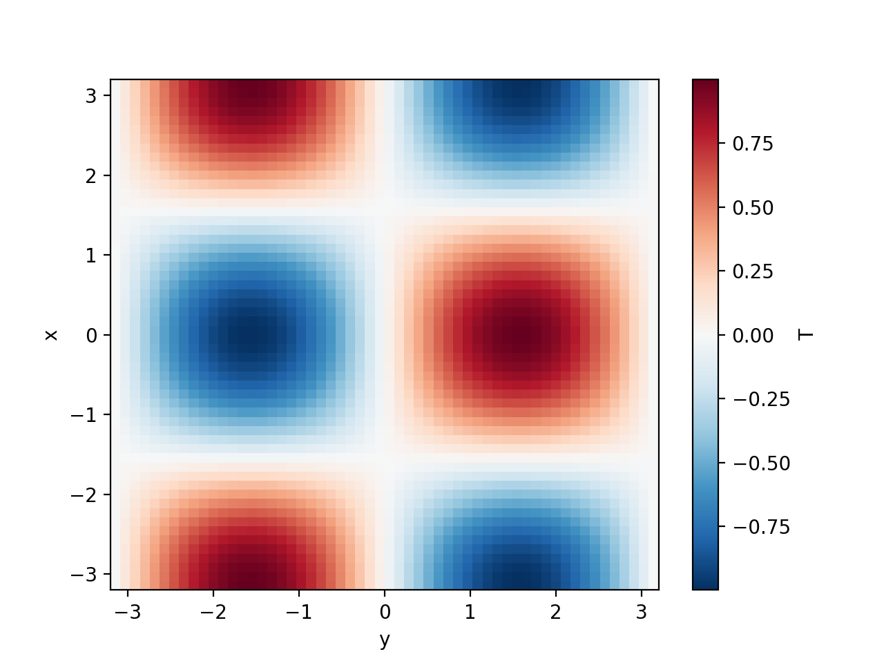
>>> T = np.cos(xx) * np.sin(yy)

>>> initial_fields = model.Fields(x=x, y=y, T=T, k=1)
>>> initial_fields["T"].plot()
<matplotlib.collections.QuadMesh object ...>

(png, hires.png, pdf)

High level simulation handler

You have the model as well as the initial condition : you are ready to launch the simulation.

The high level object in scikit-fdiff is the Simulation. It takes the model, the initial fields (as Fields or as dictionary), a time-step and some optional parameters that will feed the temporal scheme. Most of them takes at least a parameter time_stepping: bool that default to True and a parameter time_stepping: float that will drive the time stepping.

For the other solver parameters, refer to the temporal scheme page.

>>> import pylab as pl
>>> import numpy as np
>>> from skfdiff import Model, Simulation

>>> model = Model("k * (dxxT + dyyT)", "T(x, y)", parameters="k")

>>> x = np.linspace(-np.pi, np.pi, 56)
>>> y = np.linspace(-np.pi, np.pi, 56)
>>> xx, yy = np.meshgrid(x, y, indexing="ij")
>>> T = np.cos(xx) * np.sin(yy)
>>> initial_fields = model.Fields(x=x, y=y, T=T, k=1)

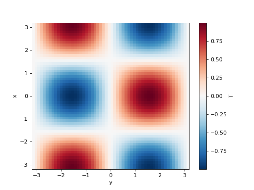
>>> simulation = Simulation(model, initial_fields, dt=0.1, tmax=1)
>>> tmax, last_fields = simulation.run()
>>> last_fields["T"].plot()
<matplotlib.collections.QuadMesh object ...>

(png, hires.png, pdf)

For better control of the simulation process, you can iterate on each time-step instead of running the simulation until you reach tmax. The Simulation object is an iterator itself that yield the tuple (t, fields) at each time step. You can then print the result, plot the fields, or do some control (stopping the simulation if something wrong happened for example).

>>> simulation = Simulation(model, initial_fields, dt=0.1, tmax=10)
>>> for t, fields in simulation:
...     print("time: %g, T mean value: %g" %
...           (t, fields["T"].mean()))
time: ..., T mean value: ...

See also

Stream Interface

How to use the Simulation.stream: Streamz.Stream interface to automate such process.

Most of the daily process are already available in the skfdiff.plugins or implemented in the Simulation:

• Post-process on the fields to compute derived fields (as flux, mean values…).

• Keep the results for some or each time-steps.

• Real time display in a jupyter notebook.

Modify the fields on the fly with the hook

You can provide a hook to the simulation (in fact, you can provide a hook the same way to the lower-level skfdiff objects as the Temporal schemes and the Routines). This hook is a callable that take the actual time and fields, and return a modified fields.

This hook will be called every time the evolution vector F or the Jacobian matrix J has to be evaluated. This can be useful to include strongly non-linear effect that would have been hard or impossible to formulate directly in the model.

Warning

Be careful with the usage of the hook: as it allows to implement complex non-linear effect, they could be source of instabilities. It is a way to do some handy hack that overcome numerical difficulties but the resulting solution will be hardly trust-able.

>>> def hook(t, fields):
...   T = fields["T"].values
...   # We bound the value of T, to be sure it does not go over 0.5
...   fields["T"] = ("x", "y"), np.where(T > 0.5, 0.5, T)
...   return fields

>>> simulation = Simulation(model, initial_fields,
...                         dt=0.1, tmax=10, hook=hook)

Keep the results in a container

A container is an object that will save the fields for each or some time-steps. It can be in-memory container (by default) or save the data in a persistent way on disk. In that case, a netCDF file will be created on disk.

The skfdiff.Container is a thin wrapper around the xarray library that will concatenate the fields of each time-steps and save it on disk if requested by the user. It has a main attributes, Container.data that return the underlying xarray.Dataset.

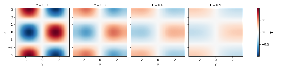
>>> simulation = Simulation(model, initial_fields, dt=0.1, tmax=1)
>>> container = simulation.attach_container() # in-memory container
>>> t, fields = simulation.run()
>>> container.data["T"].isel(t=slice(0, 10, 3)).plot(col="t")
<xarray.plot.facetgrid.FacetGrid object ...>

(png, hires.png, pdf)

For persistent container, you can retrieve the container data with the function method retrieve_container(path).

>>> from skfdiff import retrieve_container
>>> simulation = Simulation(model, initial_fields,
...                         dt=0.1, tmax=1,
...                         id="heat_diff")
>>> simulation.attach_container("/tmp/skfdiff_output/",
...                             force=True) # on-disk container
path:   ...
Empty
>>> t, fields = simulation.run()
>>> data = retrieve_container("/tmp/skfdiff_output/heat_diff")
>>> data["T"].isel(t=slice(0, 10, 3)).plot(col="t")
<xarray.plot.facetgrid.FacetGrid object ...>

To avoid to balance the memory usage and I/O call, the data are not stored on-disk every time-steps. The buffer size can be set on container creation, and is equal to 50 by default. The container will create a new file each time it store the data. These file are merged at the end of the simulation. That strategy allow the user to manipulate the results already on disk in an other script or notebook, even with a very long simulation.

If something have gone wrong and the data are not stored, you can force that with an instantiated Container container.merge(), or, using the path of the container with the static method Container.merge_datafile(path).

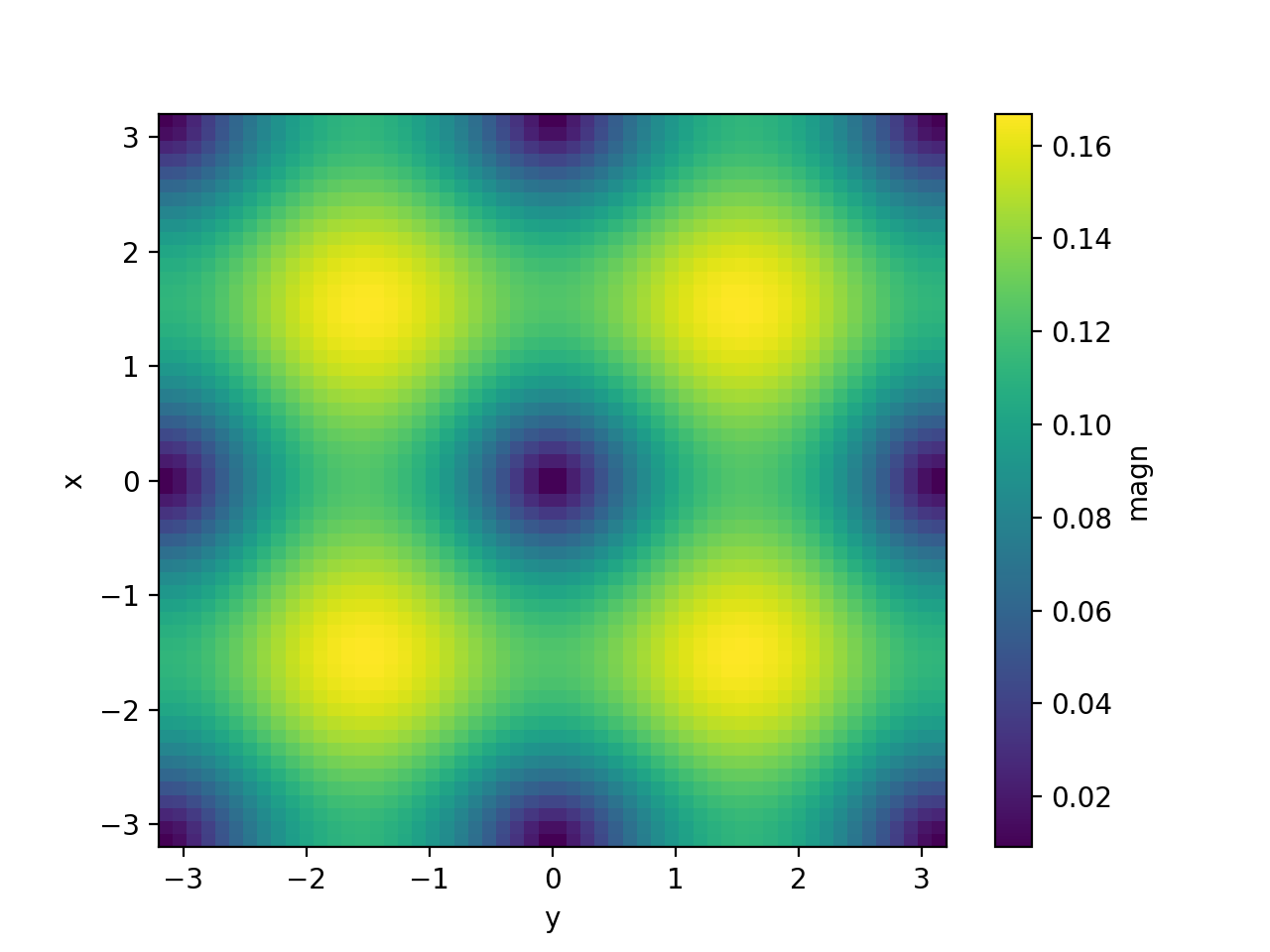
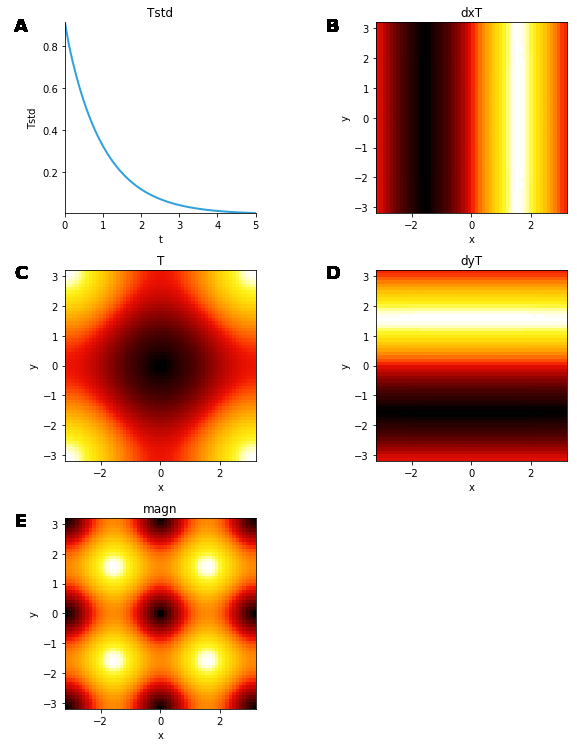
Extend your simulation with post-processes

You can add extra step after each time-steps with the post-process interface. It allows to plug a callable that take the simulation as arguments to modify the simulation state itself, or to modify the actual fields. You can use it to add some metrics to the fields (as the running time, some probes as mean values or other).

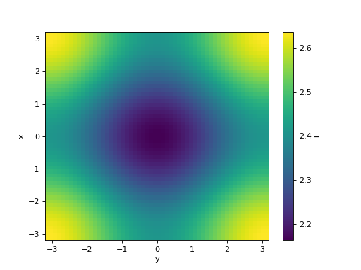
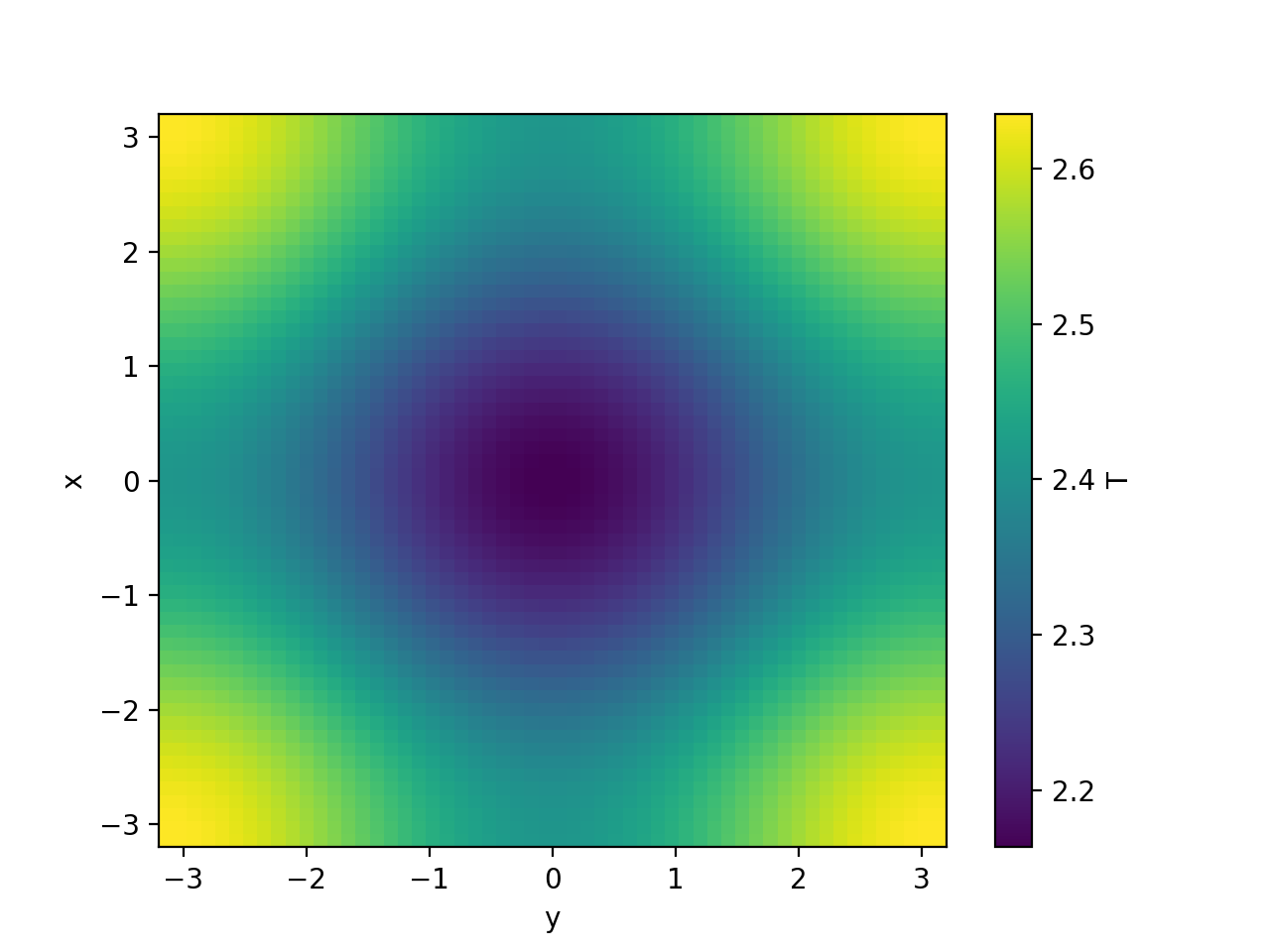
>>> import numpy as np
>>> from skfdiff import Model, Simulation
>>> model = Model("k * (dxxT + dyyT)", "T(x, y)", parameters="k")

>>> x = np.linspace(-np.pi, np.pi, 56)
>>> y = np.linspace(-np.pi, np.pi, 56)
>>> xx, yy = np.meshgrid(x, y, indexing="ij")
>>> T = np.sqrt(xx ** 2 + yy ** 2)
>>> initial_fields = model.Fields(x=x, y=y, T=T, k=1)

>>> simulation = Simulation(model, initial_fields, dt=.25, tmax=2)

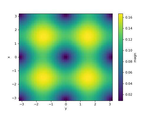
>>> def post_process(simul):
...     dxT, dyT = np.gradient(simul.fields["T"].values)
...     dx = np.gradient(simul.fields["x"].values)
...     dy = np.gradient(simul.fields["y"].values)
...     simul.fields["Tstd"] = (), simul.fields["T"].std().data
...     simul.fields["dxT"] = ("x", "y"), (dxT / dx).data
...     simul.fields["dyT"] = ("x", "y"), (dyT / dy).data
...     simul.fields["magn"] = ("x", "y"), np.sqrt(simul.fields["dxT"] ** 2 +
...                                                simul.fields["dyT"] ** 2).data

>>> simulation.add_post_process("post_process", post_process)
>>> print("Initial standard deviation: %g" % simulation.fields["Tstd"])
Initial standard deviation: ...
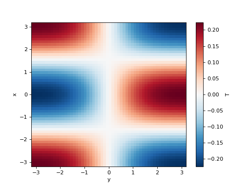
>>> t, fields = simulation.run()
>>> fig = pl.figure()
>>> simulation.fields["T"].plot()
<matplotlib.collections.QuadMesh object ...>
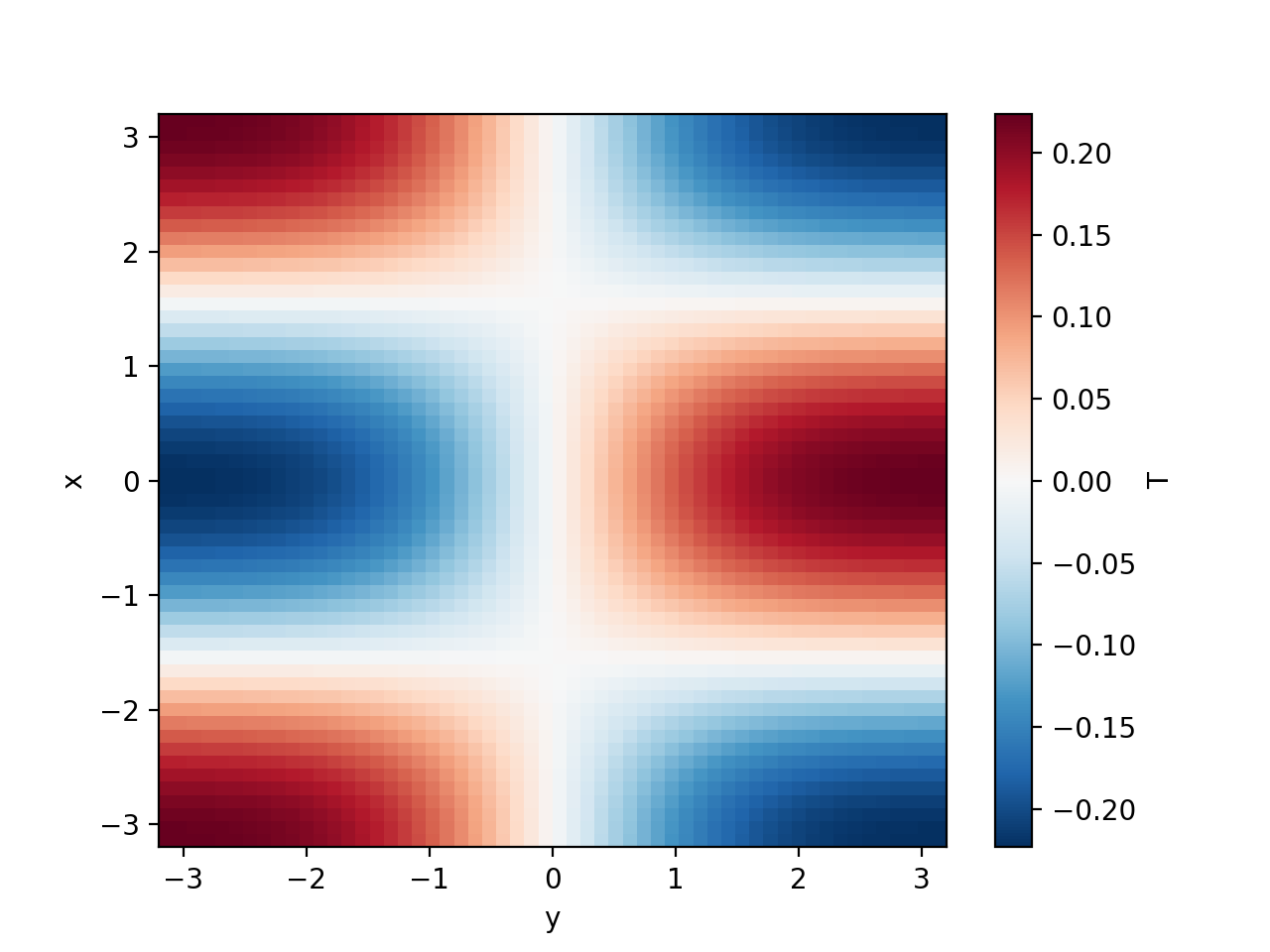
>>> fig = pl.figure()
>>> simulation.fields["magn"].plot()
<matplotlib.collections.QuadMesh object ...>
>>> print("Final standard deviation: %g" % simulation.fields["Tstd"])
Final standard deviation: ...

(png, hires.png, pdf)

(png, hires.png, pdf)

Display the result in real-time

The displays are tools that allow real-time visualisation of the data, during the simulation. For now, we only provide visualisation for the simulation running in a jupyter notebook. You can plot 1D and 2D in a straightforward manner with display_fields(), and display 0D data (often obtained via a post-process) with display_probe(). You have to run the following example in a notebook.

>>> from skfdiff import display_fields, enable_notebook
>>> enable_notebook()
>>> simulation = Simulation(model, initial_fields,
...                         dt=0.1, tmax=1)
>>> simulation.add_post_process("post_process", post_process)
>>> display_fields(simulation)
<skfdiff.plugins.displays.Display object ...>
>>> t, fields = simulation.run()

Note

We plan to provide some other, as real-time visualisation with matplotlib animation (that you can use everywhere a graphical server is available), and a cli tool that display the data from a on-disk skfdiff container.

Note

A word on the stream interface: The simulation object as a Simulation.stream: Streamz.Stream attribute that will be fed on the simulation itself at every time step. The post-process, display and container interfaces are built on it.

You can easily build complex post-process analysis by using this stream. For that, refer to the Streamz documentation.