Model¶

The skfdiff.Model object contains 5 main methods :

skfdiff.Model.F()
skfdiff.Model.J(),
skfdiff.Model.U_from_fields(),
skfdiff.Model.fields_from_U()
skfdiff.Model.Fields()

The two first are referred as model routines, the next two are provided by the grid builder while the later is an helper method that will build the xarray.Dataset adapted for the routines.

As you can easily create a Model from scratch by providing these methods. This is a way to solve a specialized problem and still have access to all the scikit-fdiff goodies. You will be able to use the scikit-fdiff Simulation even if you skip its discretisation step.

In that case, skfdiff.Model.J() is the only optional method. If you choose to skip the Jacobian computation, the implicit solvers will be unavailable.

The scikit-fdiff model transform a system of partial differential equations to the two routines skfdiff.Model.F() skfdiff.Model.J(), passing through the following steps:

transform the scikit-fdiff pseudo-language to sympy expressions

>>> from skfdiff import PDEquation
>>> pde = PDEquation("dxxU + dyyU", "U(x, y)")
>>> pde.symbolic_equation
Derivative(U(x, y), (x, 2)) + Derivative(U(x, y), (y, 2))

discretize the sympy expressions using finite difference.

>>> pde = PDEquation("dxxU", "U(x)")
>>> pde.fdiff.simplify()
(U[x_idx + 1] + U[x_idx - 1] - 2*U[x_idx])/dx**2

Apply both precedent step for each equation of the system, and do the same for the boundary conditions.
Find the domains where the different boundary condition and where the main equations have to be applied.
For each of this domain, find the symbolic condition as well as the associated discrete equation.
Build the final discrete piecewise function \(F(U_i)\) as well as the associated discrete piecewise jacobian.
Use this symbolic representation of the system to build a numerical routine that, given a Fields, will compute both \(F(U)\) and \(J(U)\). This is the role of the backends.

Skfdiff pseudo language¶

The mathematical pseudo-language used by scikit-fdiff is the same as the one understood by sympy, with some addition.

dxU will be interpreted as Derivative(U, x). It will be the same for dyyU, dxyV …
dx(U ** 2 + V) will be interpreted as Derivative(U ** 2 + V, x).doit().
Dx(U ** 2 + V) will be interpreted as Derivative(U ** 2 + V, x). This means that the derivative will not be expanded before discretisation, keeping the equation structure.

Routines¶

The two routines skfdiff.Model.F() and skfdiff.Model.J() will compute the evolution vector \(\frac{\partial U}{\partial t} = F(U)\) and its associated Jacobian matrix:

\[\begin{split}J(U) = \begin{bmatrix} \frac{\partial F_0}{\partial U_0} & \cdots & \frac{\partial F_0}{\partial U_j} & \cdots & \frac{\partial F_0}{\partial U_N} \\ \vdots & \ddots & & &\vdots\\ \frac{\partial F_i}{\partial U_0} & & \frac{\partial F_i}{\partial U_j} & & \frac{\partial F_i}{\partial U_N} \\ \vdots & & & \ddots &\vdots\\ \frac{\partial F_N}{\partial U_0} & \cdots & \frac{\partial F_N}{\partial U_j} & \cdots & \frac{\partial F_N}{\partial U_N} \end{bmatrix}\end{split}\]

Both take a fields, an optional t that default to t=0 and an optional callable hook (described in the Hook section).

Backends¶

The backends take the symbolic discrete system and build a (if possible) fast numerical routine to compute \(F\) and \(J\).

For now, two of them are implemented : the first one use numpy, the second one use numba. The last one should have better performance, but is more complex to install (conda installation is strongly recommended). It can also fail on the most complex models.

As we have access to a piecewise symbolic equation in a discrete form, we can easily build such routine, that will compute the proper value for each domain.

Grid builder¶

We take multi-dimensional array as input. The ODE solvers will work with 1D solution vector \(U\) and with 1D evolution vector \(F(U)\). We have to provide the application that transform the complex fields Dataset to a column vector : such operation is names vectorization. We also have to provide the inverse application, so called Matricization or Tensor reshaping.

We can do that in a trivial way by flattening every input array, then concatenate them. This will be good enough for explicit solvers where we only need the vector \(F(U)\). But, as we compute the associated Jacobian, we will quickly observe that this vectorization is sub-optimal. With a simple couplage between two 1D equation, the way we flatten and concatenate them will have a strong impact on the structure of the system we will have to solve.

To have a better understanding, we can implement a simple 1D system via numpy :

\[\begin{split}\begin{cases} \frac{\partial u}{\partial t} = \partial_{xx}u \times \partial_{xx}v\\ \frac{\partial v}{\partial t} = \partial_{xx}u + \partial_{xx}v \end{cases}\end{split}\]

with periodic boundary condition.

The first attempt will use a simple concatenation : we will pile up all the \(u\) then all the \(v\) as :

\[\begin{split}U = \begin{bmatrix} u_0\\ \vdots\\ u_i\\ \vdots\\ u_N\\ v_0\\ \vdots\\ v_i\\ \vdots\\ v_N \end{bmatrix}\end{split}\]

We can write some useful function, the first to approximate the jacobian matrix via finite difference (in an very inefficient way, but sufficient for teaching purpose), and the second to display the non-null entry of the jacobian matrix.

import numpy as np
import pylab as pl
import seaborn as sns
from functools import partial
from scipy.sparse import coo_matrix

def display_jac(J):
    J = (J != 0)
    if J.shape[0] < 20:
          sns.heatmap(J, cbar=False, cmap="gray_r",
                      linecolor="black", linewidths=.1, annot=True)
    else:
        J = coo_matrix(J)
        pl.scatter(J.row, J.col, color="black", marker=".")
        sns.despine(bottom=True, left=True)
        pl.gca().invert_yaxis()

def approx_fac(F, U, eps=1E-9):
    jac = np.zeros((U.size, U.size))
    eps = 1E-9
    for i in range(U.size):
        U_p = U.copy()
        U_m = U.copy()
        U_p[i] += eps
        U_m[i] -= eps
        jac[:, i] = (F(U_p) - F(U_m)) / (2 * eps)
    return jac

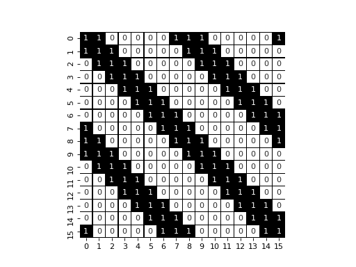
We will first try our first naive approach :

def F_naive(U, dx):
    u = U[:U.size//2]
    v = U[U.size//2:]
    dxx = lambda U: (np.roll(U, 1) - 2 * U + np.roll(U, -1)) / dx**2
    return np.concatenate([dxx(v) * dxx(u), dxx(v) + dxx(u)])

x, dx = np.linspace(-1, 1, 8, retstep=True)
u = x ** 2
v = np.cos(x)

U = np.concatenate([u, v])
naive_jac = approx_fac(partial(F_naive, dx=dx), U, eps=1E-12)

display_jac(naive_jac)
pl.axes().set_aspect('equal')

(png, hires.png, pdf)

As we can see, we have three diagonal that appears, with extra values that appears due to the periodic boundary condition.

As second attempt, we will pile up the unknowns one after the other one node at the time :

\[\begin{split}U = \begin{bmatrix} u_0\\ v_0\\ \vdots\\ u_i\\ v_i\\ \vdots\\ u_N\\ v_N \end{bmatrix}\end{split}\]

In that case :

def F_optimized(U, dx):
    u = U[::2]
    v = U[1::2]
    dxx = lambda U: (np.roll(U, 1) - 2 * U + np.roll(U, -1)) / dx**2
    return np.vstack([dxx(v) * dxx(u), dxx(v) + dxx(u)]).flatten("F")

x, dx = np.linspace(-1, 1, 8, retstep=True)
u = x ** 2
v = np.cos(x)

U = np.vstack([u, v]).flatten("F")
opt_jac = approx_fac(partial(F_optimized, dx=dx), U, eps=1E-12)

display_jac(opt_jac)
pl.axes().set_aspect('equal')

(png, hires.png, pdf)

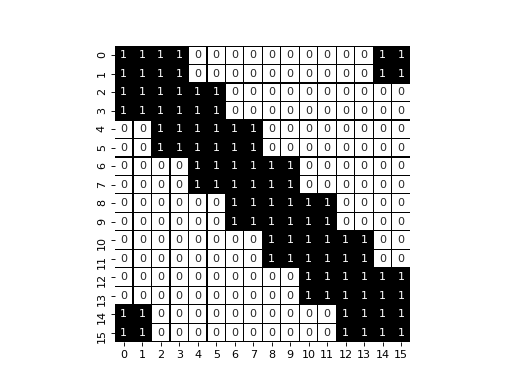
In that case, we have a larger unique band (with extra values due to the boundary condition). That structure is easier to solve by the sparse solvers available and will lead to performance improvement.

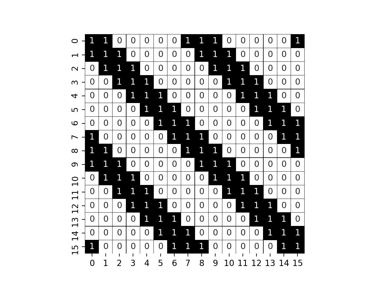
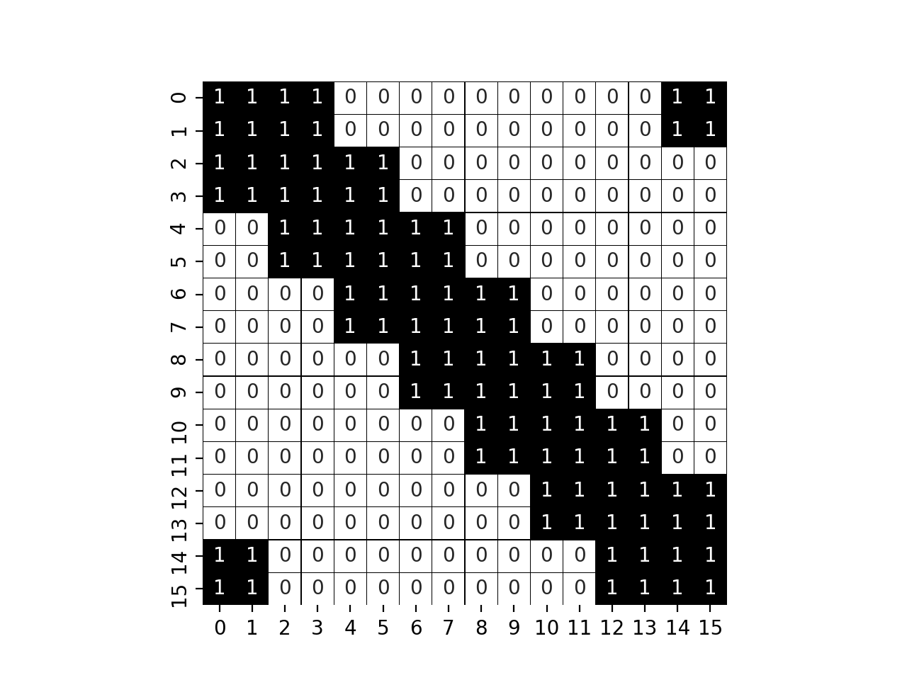
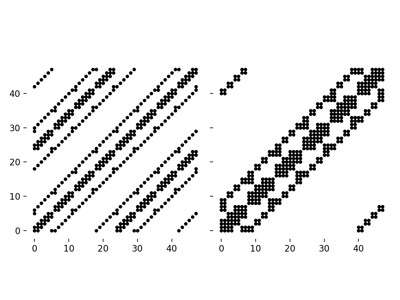
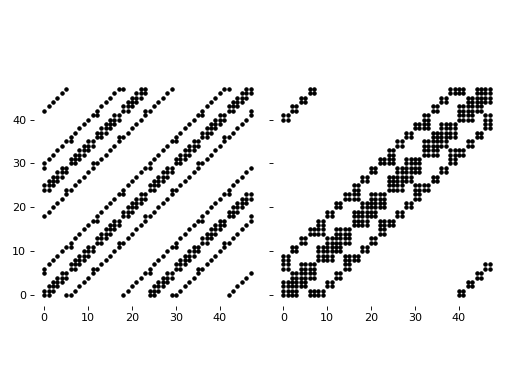
What we demonstrate for 1D coupled system will be worst for 2D problems.

For a 2D coupled system with periodic boundary condition,

\[\begin{split}\begin{cases} \frac{\partial u}{\partial t} = \partial_{xx}v \times \partial_{xx}u + \partial_{yy}v \times \partial_{yy}u\\ \frac{\partial v}{\partial t} = \partial_{xx}u + \partial_{xx}v + \partial_{yy}u + \partial_{yy}v \end{cases}\end{split}\]

we will obtain the following system, with an naive and with an optimized approach (the latter being computed with scikit-fdiff) :

from skfdiff import Model

def F_naive2D(U, dx, dy, shape):
    u = U[:U.size//2].reshape(shape)
    v = U[U.size//2:].reshape(shape)
    dxx = lambda U: (np.roll(U, 1, axis=0) - 2 * U + np.roll(U, -1, axis=0)) / dx**2
    dyy = lambda U: (np.roll(U, 1, axis=1) - 2 * U + np.roll(U, -1, axis=1)) / dy**2
    dtu = dxx(v) * dxx(u) + dyy(v) * dyy(u)
    dtv = dxx(v) + dxx(u) + dyy(v) + dyy(u)
    return np.concatenate([dtu, dtv], axis=None)

model = Model(["dxx(v) * dxx(u) + dyy(v) * dyy(u)",
               "dxx(v) + dxx(u) + dyy(v) + dyy(u)"],
              ["u(x, y)", "v(x, y)"],
              boundary_conditions="periodic")

x, dx = np.linspace(-1, 1, 4, retstep=True)
y, dy = np.linspace(-1, 1, 6, retstep=True)
xx, yy = np.meshgrid(x, y, indexing="ij")
u = xx ** 2 + np.exp(yy)
v = np.cos(xx) * np.sin(yy)

U = np.concatenate([u, v], axis=None)
jac = approx_fac(partial(F_naive2D, dx=dx, dy=dy,
                         shape=(x.size, y.size)),
                 U, eps=1E-12)

fig, (ax1, ax2) = pl.subplots(1, 2, sharey="all")
pl.sca(ax1)
display_jac(jac)

fields = model.Fields(x=x, y=y, u=u, v=v)

jac = model.J(fields).A

pl.sca(ax2)
display_jac(jac)

ax1.set_aspect('equal')
ax2.set_aspect('equal')
pl.tight_layout()

(png, hires.png, pdf)

If we compare the time spent for solving the stationary solution with the two different way to do the vectorization:

The model has to provide the routine that transform the Fields, which are a collection of multidimensional array, to a column vector, and the inverse transform : the Model.U_from_fields() and Model.fields_from_U(). The grid builder is designed to provide this two methods in a way that optimize the jacobian structure in a way that improve the solving of the resulting linear system.